Chapter 7. Trading Systems
Prev		Next

Chapter 7. Trading Systems

Table of Contents

1. General Information

1.1. Introduction

The purpose of a trading system is to define a buying and selling strategy based on conditions established from technical indicators, and to test its profitability on historical prices to derive the decision rules to be applied in the future.

This approach is based on the postulate that in the future, prices will generally exhibit the same behaviors as they did in the past. This is partially true, but with two important remarks:

The profitability of a strategy can change significantly after certain periods. It is therefore necessary to verify it regularly to determine if the buying and selling conditions are still current or if they deserve to be revised.
Instruments do not all behave the same way. Therefore, good strategies are not suitable for all instruments.

Axial Finance allows for the simple design of even complex strategies, analyzing their profitability and loss risks in detail, comparing them with each other, and identifying the instruments for which they are best suited.

1.2. Definition of important terms

This chapter frequently uses the following terms, which should be understood as follows:

Bar	The time unit of a chart. For example, in a daily chart, a bar represents one trading session. In a 5-minute intraday chart, the bar represents a 5-minute time unit.
Indicator	A numerical function evolving over time (bar after bar) representable graphically by a curve. Technical indicators are indicators specifically developed for technical analysis.
Signal	An elementary TRUE or FALSE condition, determined at each bar based on the use of indicators. Example of a signal: "The closing price crosses above a Moving Average".
Rule	A logical combination of signals, defining a complex condition evaluated as TRUE or FALSE. A signal can be considered a simple rule composed of a single condition.
Stop	A position closing condition that takes priority over the closure rule if one is present. For example, a stop for closing a position when the loss recorded since the opening of the position exceeds a certain threshold.
Modalities	The set of modalities allowing the evaluation of a strategy's profitability. For example, the initial stake, the maximum number of shares per trade, etc.
Strategy	A strategy is characterized by its opening and closing rules, potentially by stop conditions, and by its modalities for evaluating results.
Long position	A position is said to be "long" when it is opened by buying shares and closed by selling those shares.
Short position	A position is said to be "short" when it is opened by the short sale of shares and closed by repurchasing those shares.
Backtesting	The operation consisting of applying a strategy to a historical price series.
Equity curve	The bar by bar value of the capital invested starting from an initial stake resulting from the application of a strategy.
Drawdown	The eventual loss recorded upon position closure. The maximum drawdown defines the maximum loss recorded during various trades. The maximum drawdown therefore measures the maximum risk of loss of a strategy.

1.3. Implementation

The set of operations that can be performed in the implementation of trading systems are as follows:

Programming personal indicators using the universal programming language JavaScript for use in signals
Programming of signals using the universal programming language JavaScript for use in rules
Designing rules for buying and selling to be used in strategies or in market screening (in which case we speak of a screening rule)
Designing trading strategies and performing backtesting on a price chart (daily or intraday).
Displaying the equity curve in a chart window of the Market Tracking area along with position opening and closing signals
Displaying the drawdown in the chart
Displaying equity curves in the Strategy Screen module as an alternative to Market Tracking. Strategy Screen allows for the simultaneous calculation and display of results:
- of the same strategy applied to a list of stocks
- of a list of strategies applied to the same stock
- a single strategy applied to a stock while varying certain parameters of the rules step by step
Selecting the vertical scale of the equity curve in monetary amount or as a relative percentage of gain/loss
Selecting the presentation of the equity curve with or without the potential variations during position opening
Presenting the detailed result of a strategy with a global summary, the list of open positions, and the values of the equity curve
Presenting in a summary table the full set of results for all executed strategies
Exporting and importing software personal indicators, signals, and strategies
Exporting open positions of a strategy and the equity curve to an Excel file.

2. Creating strategies

2.1. Generalities

A strategy is defined by:

its opening and closing position rules
eventually position closing stop conditions
its modalities for evaluating profitability

Important

Before creating a strategy, ensure that all signals and rules necessary for defining the opening and closing conditions exist in the library. If not, begin by defining them as explained in the paragraphs below: Indicator Programming and Signal Programming.

2.2. Creation

To create or modify a strategy, in the general Trading System menu, choose the Strategies option to open the editing window:

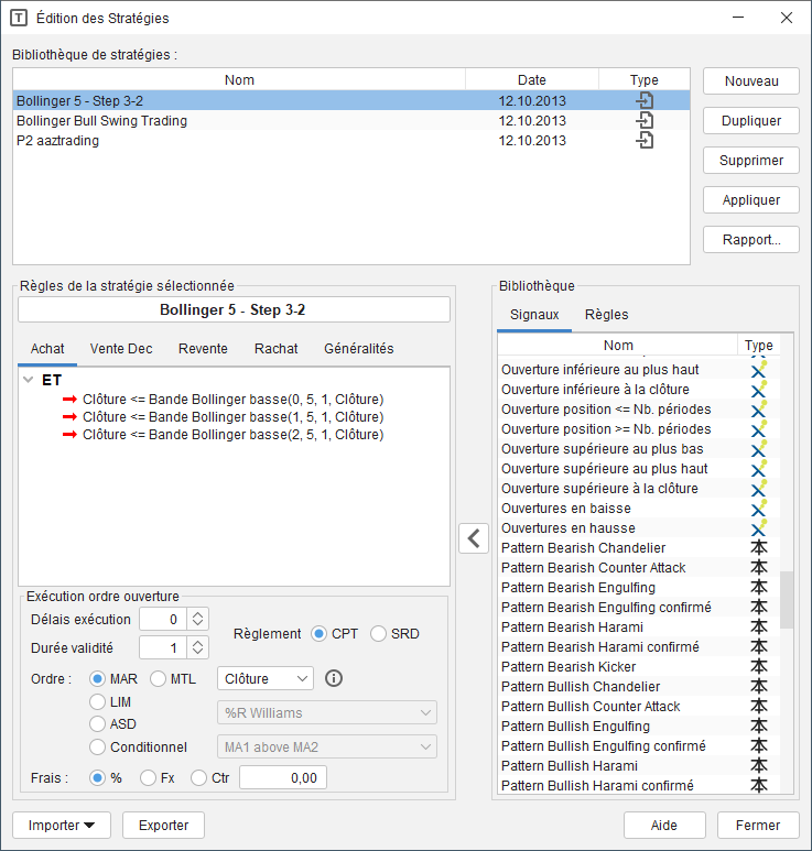
The editing window comprises three parts:

At the top, the list of strategies in the library and to its right the buttons New, Copy, Delete, Apply, and Report...
In the center left, an area with a tab box, displaying for the strategy selected in the library above:
- The name
- In the Buy tab: the "long" opening rule with order execution conditions
- In the Short Sale tab: the "short" opening rule with order execution conditions
- In the Sell tab: the "long" closing rule with order execution conditions
- In the Cover tab: the "short" closing rule with order execution conditions
- In the General tab: the modalities of the order (initial stake, number of shares per order, etc.)
In the center right, the list of signals and rules in the library for composing the opening and closing rules of the strategy.

By clicking on the New button, a new strategy is added to the library under the temporary name "(New)". Enter the name of this strategy in this field and then define the rules, execution conditions, and modalities as explained below.

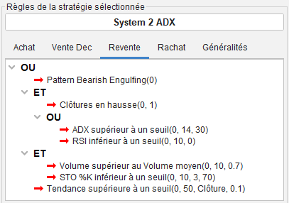
2.3. Creation of position opening and closing rules

A strategy can include:

Two rules: long opening and long closing
Two rules: short opening and short closing
Four rules: long opening, long closing, short opening, and short closing

To each rule, execution conditions are associated, just as when placing an order with a broker.

The procedure for creating a rule is identical to that described in the paragraph Creation and editing of rules.

Then for each rule:

2.3.1. Defining the root condition

Each rule must start with an initial condition called the root condition. By default, this condition is an (AND in Boolean logic).

To replace the root condition AND with an OR, right-click on the root condition icon to open the context menu and choose the option Replace AND with OR.

Proceed inversely with Replace OR with AND.

2.3.2. Inserting a signal

To add a signal to the root condition or to any other condition or of the rule:

Right-click on the condition icon and open the context menu, then choose the option Add signal. A red horizontal arrow prefiguring the place of the signal is inserted below.
Select this red arrow by clicking on it.
To subsequently insert a signal from the library, two methods are available:
1. select the signal from the list and click on the button
2. or drag this signal with the left mouse button, hold it, and release the mouse button over the red arrow.

2.3.3. Parameterizing a signal

To parameterize a new signal added by the previous method, or to modify the parameters of an existing signal:

Double-click on the signal in the graphical representation of the rule to open the parameter entry window.
Define the various parameters and then click the OK button.

2.3.4. Changing a signal

To replace a signal in the rule with another signal from the library:

Select the signal to be replaced by clicking on it in the graphical representation of the rule.
Then, two methods are available:
1. Select the new signal from the library and click on the button
2. or drag this signal with the left mouse button, hold it, and drop the pointer over the arrow in the graphical representation.

2.3.5. Adding AND / OR conditions

The addition of an AND or OR condition is performed from the position of a signal in the graphical representation at the logical location (in terms of Boolean logic) of the future condition.

Select the signal that is at the logical position of the condition to be added.
Click on the arrow of this signal and then open the context menu by right-clicking it.
Depending on the case, choose the option Replace with OR or Replace with AND.

Example of constructing a complex rule:

2.3.6. Replacing an AND / OR condition

To replace one condition with another condition:

Click on the image of this condition and then open the context menu by right-clicking it.
Depending on the case, choose the option Replace with OR or Replace with AND.

2.3.7. Deleting a signal or a condition

Click on the image of this condition or signal and then open the context menu by right-clicking it.
Choose the option Cancel.

Deleting a condition deletes all signals and other conditions included in that condition.

2.4. Defining execution conditions

For each position opening and closing order, precise execution conditions can be set:

2.4.1. Execution delay

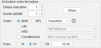
The order can be executed on the bar of the signal or on a subsequent bar. Thus, in a daily chart, to execute an order the next day, one displays the value 1 for the execution delay, otherwise 0 for immediate execution.

2.4.2. Validity duration

When an order is initialized after a signal, its execution depends on the execution condition depending on the type of order. Depending on the case, execution can be immediate or deferred in waiting for the realization of the condition. The validity duration defines the number of bars during which the initialized order can be executed; otherwise, if this delay is exceeded, the order will be cancelled.

A validity delay equal to 1 in an ongoing "end of day" chart means that the order can only be executed for one single day.

2.4.3. Order type

Axial Finance allows choosing between the following four order types, which are generally available at brokers:

Market	the order will be executed immediately at the price of the bar defined in the associated drop-down list: Open, Close, etc.
Best Limit (ML)	To define the best limit price, one chooses from the associated drop-down list a technical indicator that calculates this limit price at the execution bar. For example, to set the limit price at 1% below the opening price of the bar, it is sufficient to create an indicator performing this calculation, which is then selected in the drop-down list.
Stop Limit (ASD)	To define the trigger threshold price, one chooses from the associated drop-down list a indicator that calculates this trigger price at the execution bar. For example, to set the trigger price at 2% above the opening price of the bar, it is sufficient to create an indicator performing this calculation, which is then selected in the drop-down list.
Conditional	A more complex execution condition can be defined, for example, if the price goes above the 30-period moving average. One creates in the library the rule corresponding to the desired condition, which is then selected from the associated drop-down list of the condition.

2.4.4. Brokerage fees

Brokerage fees can be defined in three different ways:

%	as a percentage of the order amount.
Fx	as a fixed amount per order.
Ctr	as a fixed amount per number of shares (or contracts).

2.5. Definition of stop conditions

Independently of the position closing conditions defined in the rules, Axial Finance allows deciding without waiting for the closure of a "long" or "short" position in certain specific situations.

To program these situations, click on the Stops button to open the dialog box. Seven types of stop can be activated:

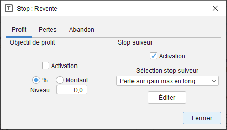Stop if the Profit target is reached

This stop is activated by checking the Activation box. The profit target level is set in Amount or as a % of the opening price. Enter the profit level in the Level field.

Stop when the Trailing stop level is breached.

This stop is activated by checking the Activation box. A trailing stop allows defining the price level to close the position at each period. This level is recalculated at each period based on a formula defined by the user. This formula is equivalent to programming a personal indicator. Click on the Edit button to open the dialog box for programming this formula and then select its name from the drop-down list to assign it to the trailing stop.

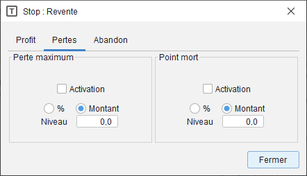Stop if the position reaches a Maximum loss level.

This stop is activated by checking the Activation box. The maximum loss level for the position is set in Amount or as a % of the opening price. Enter the loss level in the Level field.

Stop if the Break even is reached.

This stop is activated by checking the Activation box. It triggers when the price returns near the opening price. The break-even threshold is set in Amount or as a % of the opening price. Enter the break-even threshold in the Level field.

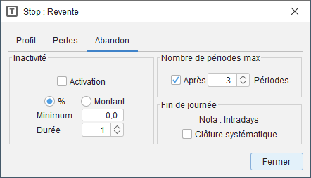Stop in case of Inactivity.

This stop is activated by checking the Activation box. It allows avoiding keeping a position open if the price does not evolve sufficiently during a certain duration. Check the corresponding boxes in the Inactivity frame and enter the numerical value (in % or amount) of the Minimum threshold to be exceeded, as well as the number of periods defining the duration since the opening of the position.

Stop after a Max number of periods.

This stop is activated by checking the After box. It allows systematically closing a position after a fixed number of periods if the position is still open. Define in the Periods drop-down list this maximum number of periods for the position opening.

Stop at End of day (intraday case)

Check the box in the corresponding frame to activate this stop mode applied only in the case of intraday charts.

2.6. Defining Modalities

Select the General tab and specify the following modalities for the application of the strategy:

2.6.1. Starting capital

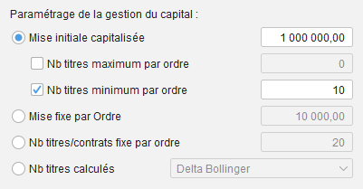
Four different methods can be used to define the number of shares at position opening:

Capitalized initial stake	At each position opening, Axial Finance determines the maximum number of shares that can be bought (or sold) based on the available capital and the current price. Upon position closure, the available capital is updated according to the profit or loss realized. The amount to enter for this method corresponds to the capital available for the first position opening. It is also possible to impose: A maximum number of shares per order. A minimum number of shares per order. Thus, no order will be executed if the available capital is insufficient.
Fixed stake per order	The capital available at position opening is always the same. Axial Finance determines the maximum number of shares that can be bought (or sold) based on this available capital and the current price.
Fixed number of shares or contracts per order	The quantity of shares or contracts bought (or sold) is always the same.
Calculated number of shares	The quantity of shares is calculated at each opening from a programmable mathematical formula. This programming is performed using a personal indicator, where the indicator value at the position opening bar must be equal to the number of shares.

In the second and third methods, for the calculation of the strategy result, Axial Finance determines retrospectively the initial capital that would have been necessary to maintain a positive or zero available capital at all times.

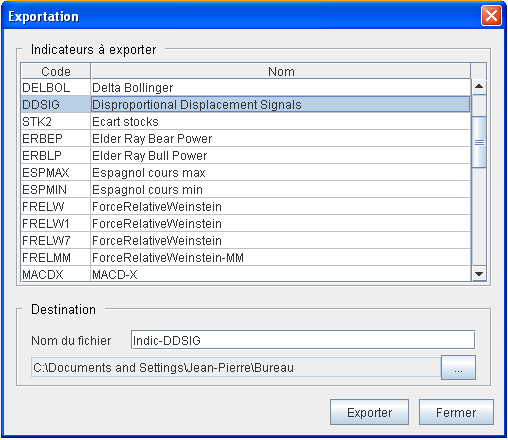
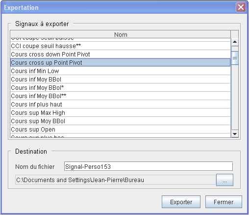
2.7. Importing and exporting strategies

Axial Finance allows for the importing and exporting of strategies between users of the software. These exchanges are performed using files transmitted via the Internet.

2.7.1. Exporting a strategy

In the general Trading System menu, choose the options Export then Strategy to open the dialog window shown here.
Select the strategy to export from the list
In the File name field, keep the default name set by the software or choose another name for the exported file.
Click on the ... button to open the destination directory selection window where the file will be saved, then click on the Choose button.
Then click on the Export button.

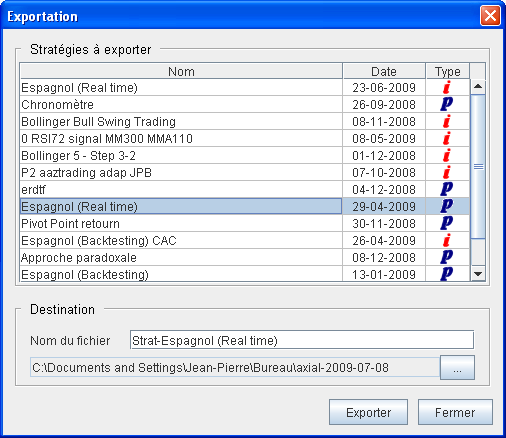The created file has the extension .strax and appears in the destination directory under the full name filename.strax.

The indicators and personal signals included in the strategy will be exported simultaneously in the same file.

2.7.2. Importing a strategy

The strategy file to be imported is saved on the computer's drive or on a USB flash drive:

In the general Trading System menu, choose the options Import from file then Strategy to open the dialog window shown here.
In the search window, select the directory and then the file to import, which must have the extension .strax.
Click on the Import button.

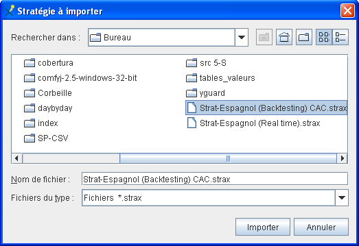In the strategies library, imported strategies are identified by the symbol

3. Programming indicators

3.1. Generalities

An indicator (or technical indicator) defines the evolution over time of a variable characterizing the state of a stock or market. There are many indicators created by analysts, generally classified into the following categories:

Trend indicators
Momentum indicators
Volatility indicators
Volume indicators
Market indicators
Support-resistance indicators

However, each user may be required to design other indicators, called personal indicators, for use in signals.

Axial Finance is provided with a library containing many indicators and also allows programming personal indicators or importing indicators designed by other users of the software.

3.2. Library of available indicators

Each indicator is defined by a unique code used in the programming of other indicators and signals.

3.2.1. Indicators from technical analysis:

Code	Name	Script
`AROdown`	Aaron Indicator down	AROdown(n, Periode)
`AROup`	Aaron Indicator up	AROup(n, Periode)
`AROosc`	Aaron Oscillator	AROosc(n, Periode)
`ADI`	Accumulation Distribution Index	ADI(n)
`ADWP`	Accumulation Distribution Williams	ADWP(n)
`ASI`	Accumulation Swing Index	ASI(n)
`ADX`	Average Directional Index	ADX(n, Periode)
`ATR`	Average True Range	ATR(n, Periode)
`BBB`	Lower Bollinger Band	BBB(n, Periode, StDev, Type)
`BBH`	Upper Bollinger Band	BBH(n, Periode, StDev, Type)
`COG`	Center of Gravity	COG(n, Periode, Prix)
`CMF`	Chaikin Money Flow	CMF(n, Periode)
`COS`	Chaikin Oscillator	COS(n, PeriodeCt, PeriodeLt)
`CVO`	Chaikin Volatility	CVO(n, Periode)
`CMO`	Chande Momentum Oscillator	CMO(n, Periode)
`CRL`	Linear Regression Curve	CRL(n, Periode, Type)
`CRP`	Close Range Position Index	CRP(n, Periode)
`CCI`	Commodity Channel Index	CCI(n, Periode)
`CSI`	Commodity Selection Index	CSI(n, Periode)
`PRX`	Price (close, open, high, ...)	PRX(n, Type)
`PRXH`	Heikin Ashi Price (close, open, high, ...)	PRXH(n, Type)
`CLO`	Closing price	CLO(n)
`OPEN`	Opening price	OPEN(n)
`HIGH`	Highest price	HIGH(n)
`LOW`	Lowest price	LOW(n)
`DPO`	Detrended Price Oscillator	DPO(n, Periode)
`DXm`	Directional Indicator Minus	DXm(n, Periode)
`DXp`	Directional Indicator Positive	DXp(n, Periode)
`DEMA`	Double EMA	DEMA(n, Periode)
`EOM`	Ease Of Movement	EOM(n)
`FIX`	Force Index	FIX(n, Periode)
`KAGI`	KAGI (see note below)	KAGI(n, Mode, Seuil)
`KBB`	Upper Keltner Band	KBB(n, Periode, Variation)
`KBH`	Lower Keltner Band	KBH(n, Periode, Variation)
`KLO`	Klinger Oscillator	KLO(n, PeriodeCt, PeriodeLt, PeriodeTr)
`MACD`	Moving Average Convergence Divergence	MACD(n, PeriodeCt, PeriodeLt)
`MACDH`	MACD - Trigger	MACDH(n, PeriodeCt, PeriodeLt, PeriodeTr)
`MASI`	Mass Index	MASI(n, Periode, PeriodeEMA)
`MINL`	Minimum Lows	MINL(n, Periode)
`MAXH`	Maximum Highs	MAXH(n, Periode)
`MOM`	Momentum	MOM(n, Periode)
`MFI`	Money Flow Index	MFI(n, Periode)
`MMAR`	Arithmetic Moving Average	MMAR(n, Periode, Type)
`MMEX`	Exponential Moving Average	MMEX(n, Periode, Type)
`MMPD`	Weighted Moving Average	MMPD(n, Periode, Type)
`MMTR`	Triangular Moving Average	MMTR(n, Periode, Type)
`MMVA`	Volume Adjusted Moving Average	MMVA(n, Periode, Type)
`MMVR`	Variable Moving Average	MMVR(n, Periode, Type)
`MMVH`	MMVH	MMVH(n, Periode)
`MMT3T`	T3 Tilson Moving Average	MMT3T(n, Periode, Ratio)
`NVI`	Negative Volume Index	NVI(n)
`OBV`	On Balance Volume	OBV(n)
`OCV`	Open-Close Volatility Index	OCV(n, Periode)
`ORP`	Open-Range Position Index	ORP(n, Periode)
`OSC`	Moving Average Oscillator	OSC(n, Periode1, Periode2, Type)
`ORL`	Linear Regression Oscillator	ORL(n, Periode, Type)
`PCRW`	%R Williams	PCRW(n, Periode)
`PRF`	Performance Index	PRF(n, Type)
`PVI`	Positive Volume Index	PVI(n)
`POSC`	Price Oscillator	POSC(n, PeriodeCt, PeriodeLt)
`PROC`	Price Rate Of Change	PROC(n, Periode)
`PRL`	Relative Prices (or Relative Strength)	PRL(n, Valeur)
`PVT`	Price and Volume Trend	PVT(n)
`QSI`	Q-Stick Indicator	QSI(n, Periode)
`RWIhigh`	Random Walk Index High	RWIhigh(n, Periode)
`RWIlow`	Random Walk Index Low	RWIlow(n, Periode)
`RVO`	Range Volatility Index	RVO(n, Periode)
`RMI`	Relative Momentum Index	RMI(n, Periode, Ecart)
`RSI`	Relative Strength Index	RSI(n, Periode)
`RVI`	Relative Volatility Index	RVI(n, Periode)
`SAR`	Parabolic SAR	SAR(n, MaxRatio, PcAccel)
`SWR`	Schwager Volatility Ratio	SWR(n, Periode)
`SPR`	Spread	SPR(n, Valeur, Ratio)
`SPTR`	Super Trend	SPTR(n, Periode, Type, Prix, Ratio)
`STD`	Standard Deviation	STD(n, Periode)
`STOD`	Stochastics %D	STOD(n, Periode, PeriodeK, PeriodeD)
`STOK`	Stochastics %K	STOK(n, Periode, PeriodeK)
`SWI`	Swing Index	SWI(n)
`TREND`	Trend Ratio	TREND(n, Periode, Type)
`TVI`	Trade Volume Index	TVI(n, Mindev)
`TEMA`	Triple EMA	TEMA(n, Periode)
`TRIX`	TRIX Indicator	TRIX(n, Periode)
`TSI`	True Strength Indicator	TSI(n, Periode1, Periode2)
`VHF`	Vertical Horizontal Filter	VHF(n, Periode)
`VOR`	Volatility Ratio	VOR(n, Periode)
`VOL`	Closing Volume	VOL(n)
`VOS`	Volume Oscillator	VOS(n, PeriodeCt, PeriodeLt)
`VROC`	Volume Rate Of Change	VROC(n, Periode)
`WUO`	Ultimate Oscillator	WUO(n, PeriodeCt, PeriodeMt, PeriodeLt)
`LVLR`	Resistance Level	LVLR(n, Rang)
`LVLS`	Support Level	LVLS(n, Rang)

Note

To define the different states of the KAGI indicator, the convention adopted is as follows: It returns the numerical value +2 in case of an upward reversal, -2 in case of a downward reversal, +3 in case of moving from upward to downward pressure, -3 in case of moving from downward to upward pressure, otherwise +1 when pressure is increasing and -1 when pressure is decreasing.

3.2.2. Date and time functions:

`YEAR`	Year	YEAR(n)
`HOUR`	Hour	HOUR(n)
`DAYW`	Day of the week	DAYW(n)
`DAYM`	Day of the month	DAYM(n)
`MONTH`	Month of the year	MONTH(n)

3.2.3. Indicators from Fundamental Analysis:

`ACNA`	Net Asset per Share	ACNA(n)
`BPAA`	Earnings per Share	BPAA(n)
`CPPR`	Equity	CPPR(n)
`CHAF`	Revenue	CHAF(n)
`DTNT`	Net Debt	DTNT(n)
`EBIT`	EBIT	EBIT(n)
`PER`	Price Earning Ratio	PER(n)
`CAPI`	Capitalization Ratio	CAPI(n)
`RNET`	Net Income	RNET(n)

3.2.4. Indicators relative to strategy positions:

These indicators are used only for the programming of the opening and closing rules of a strategy.

`DAOP`	Number of bars since opening	DAOP(n)
`DCP`	Number of bars since closure	DCP(n)
`DDSC`	Number of bars since the closure signal	DDSC(n)
`DDSO`	Number of bars since the signal of opening	DDSO(n)
`POP`	Opening price	POP(n)
`TISC`	Price at the closure signal	TISC(n, Type)
`TISO`	Price at the opening signal	TISO(n, Type)
`HCLOSE`	Closing hour	HCLOSE(n)
`HOPEN`	Opening hour	HOPEN(n, Type)

3.2.5. Library

To access the indicators library, in the general Trading System menu, choose the option Indicators. The window below opens:

Each indicator is defined by its code, its name, its script, its variable parameters and an optional comment.

3.3. Programming a personal indicator

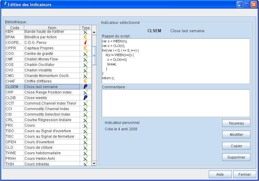
To program a personal indicator, open the window above and then click on the New button to open the entry window below.

Important

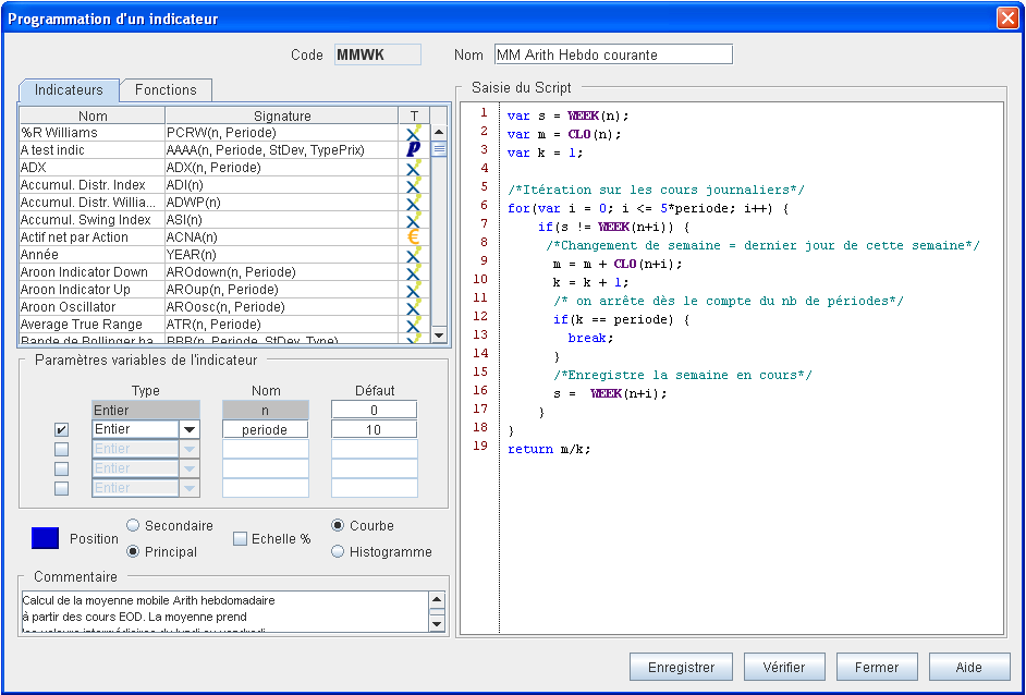
A manual explaining how to program in JavaScript is available on the website www.axialfinance.com

Enter the code of the indicator. This code is unique and will be used to reference this indicator. This code must contain at least 4 characters, letters or numbers only. Axial Finance will refuse entry if this code is already in use or if the entry is non-compliant. This code cannot be modified later. If needed, you should first cancel the indicator then reprogram it with a different code.
Enter the name of the indicator.
Enter the JavaScript program in the Script entry area. To include an indicator or a mathematical function from the library in the script, simply double-click on the name of this element in the library after placing the cursor in the script at the exact place where it should be written.

The script includes two types of variables: internal variables that can only be changed by modifying the script, and external variables that the user will have the ability to vary later (for example, the period of the indicator) without changing the programming.

Internal variables are defined in the body of the JavaScript program with the reference var: example "var sum = 0"

External variables are designated by their name in the script and defined with a type and a default value in the Indicator variable parameters area located below the library.

A indicator can include a maximum of 5 external variables, including the mandatory parameter n which defines the bar for calculation. Generally, this parameter n remains at zero, signifying that the indicator should be evaluated at the current bar. However, in some cases, one may want to offset the bar for calculation. By convention, n+1 will correspond to a delay of one bar, n+2 to a delay of two bars, etc. Consequently, if in a script the time must be rolled back by one bar for a function, one should use n+1 instead of n as the parameter value.

The reference to time is dependent on the periodicity of the prices used for calculation. Thus, with daily charts, n+1 corresponds to a one-day delay. If the same indicator is used with intraday 5-minute charts, n+1 corresponds to a 5-minute delay, etc.

The names of the external variables (other than n) are defined by the user. Each name must be unique. All external variables in the script must be defined in the Indicator variable parameters area using the same name as in the script (it is imperative to respect uppercase and lowercase characters). A default value is automatically provided, but the effective value of the variable will be that defined by the user when using this indicator in a signal, a rule, or a strategy.

Different types of variables:

Integer	Whole number
Real	Real number
Price	Nature of the price: open, high, ...
Mov.Avg.	Nature of the moving average: arithmetic, exponential, ...
Instrument	The code of an instrument
Mode	A currency or a %
Text	Alphanumeric characters

By convention, among the 4 available external variables, an indicator can include a maximum of the following types:

One Real
In addition to the variable n, three Integer if there is no variable defined as a Real, otherwise two Integer.
One variable of type Text or Mov.Avg. or Price or Instrument or Mode

Axial Finance will refuse variables if this convention is not respected. To add or remove an external variable, check or uncheck the checkbox for that line.

By convention, the last line of the script must return the result of the indicator calculation. This result must be the calculated numerical value.
To verify that the script is correct according to the JavaScript language, click on the Verify button. In case of a programming error, a message indicates the erroneous line.
Click on the Save button to save this indicator in the library. It will appear with the symbol
To modify a personal indicator, select it in the Indicator Editing window and click on the Modify button. Only the code of the indicator cannot be modified.
To delete a personal indicator, select it in the Indicator Editing window and click on the Delete button. Deletion will be refused if this personal indicator is present in a signal or a strategy.

3.4. Graphical representation of a personal indicator

When programming a personal indicator, you must specify how to display it on a chart. In the programming window, below the Variable indicator settings frame, you can define:

Plotting in the main chart of prices or in a secondary chart of a chart window. Check the corresponding case: Primary or Secondary.
The color of the curve representing the indicator. Click on the color button to open the palette of choices.
The vertical scale in units or as a percentage. Check the % box for the second choice.
Plotting in the form of a continuous curve or in the form of a histogram. Check the corresponding case: Curve or Histogram.

3.5. Mathematical Functions

A library of mathematical functions is available for the programming of indicators. It includes classic mathematical functions (example: ACOSINE(n), LOG(n), MAX(f,g), etc.) and the following technical analysis specific functions:

`MOVA(FCT,n,p,q,r,t)`	Arithmetic Moving Average
`MOVE(FCT,n,p,q,r,t)`	Exponential Moving Average
`MOVP(FCT,n,p,q,r,t)`	Weighted Moving Average
`SLOPE(FCT,n,p,q,r,t)`	Slope of the Linear Regression Line

For these specific functions, the meaning of the parameters is as follows:

`FCT`	Code of the indicator for calculating the moving average or the slope of the linear regression line
`n`	Time parameter
`p`	Calculation period of the moving average or the slope of the linear regression line
`q,r,t`	3 parameters available in case the indicator defined by the code `FCT` requires it. Unused parameters remain present in the formula but do not need to be defined

3.6. Importing and exporting personal indicators

Axial Finance allows for the importing and exporting of personal indicators between users of the software. These exchanges are performed using files transmitted via the Internet.

3.6.1. Exporting an indicator

In the general Trading System menu, choose the options Export then Indicator to open the dialog window shown here.
Select the indicator to export from the list.
In the File name field, keep the default name set by the software or choose another name for the exported file.
Click on the ... button to open the destination directory selection window where the file will be saved, then click on the Choose button.
Then click on the Export button.

The created file has the extension .indax and appears in the destination directory under the full name filename.indax.

3.6.2. Importing an indicator

The indicator file to be imported is saved on the computer's hard drive or on a USB flash drive:

In the general Trading System menu, choose the options Import from file then Indicator to open the dialog window shown here.
In the search window, select the directory and then the file to import, which must have the extension .indax.
Click on the Import button.

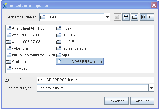In the indicators library, imported indicators are identified by the symbol

4. Programming signals

4.1. Generalities

A signal defines the TRUE or FALSE state of a condition at each bar.

The signal is the basis of the opening and closing rules, each rule corresponding to a logical combination of signals. A signal can therefore be defined as the elementary condition used to compose a rule.

Axial Finance is provided with a library of signals called native signals corresponding to the most frequently used signals. One can program and add other signals to the library, called personal signals, or import signals programmed by other users of the software.

4.2. Library of signals

To access the signals library, in the general Trading System menu, choose the option Signals to open the window below.

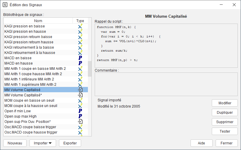
Each signal is defined by its name, its script, its variable parameters and eventually a comment. Native signals are identified by the icon .

4.3. Programming a personal signal

To program a personal signal, open the previous window and then click on the New button to open the entry window below:

Important

A manual explaining how to program in JavaScript is available on the website www.axialfinance.com

Enter the name of the signal. This name can be modified later if needed.
Enter the JavaScript program in the Script entry area defining the signal. To include an indicator or a mathematical function from the library in the script, simply double-click on the name of this element in the library after placing the cursor in the script at the exact place where it should be written.

Internal variables are defined in the body of the JavaScript program with the reference var: example "var sum = 0"

External variables are designated by their name in the script and defined with a type and a default value in the Signal variable parameters area located below the library.

A signal can include any number of external variables. All external variables in the script must be defined in the Signal variable parameters area using the same name (it is imperative to respect uppercase and lowercase characters). A default value is automatically provided, but the effective value of the variable will be that defined by the user when using this signal in a rule or a strategy.

To add an external variable to the list, click on the Add button.
To remove an external variable from the list, select it and then click on the Delete button.
To modify an external variable, select it and then click on the Modify button.

Different types of variables:

Integer	Whole number
Real	Real number
Price	Nature of the price: open, high, ...
M.A.	Nature of the moving average: arithmetic, exponential, ...
Instrument	The code of an instrument
Mode	A currency or a %
Text	Alphanumeric characters

By convention, the last line of the script must return the result of the signal evaluation. This result must be a boolean value TRUE or FALSE.
To verify that the script is correct according to the JavaScript language, click on the Verify button. In case of a programming error, a message indicates the erroneous line.
Click on the Save button to save this personal signal in the library. It will appear with the symbol
To modify a personal signal, select it in the Signal Editing window and click on the Modify button.
To delete a personal signal, select it in the Signal Editing window and click on the Delete button. Deletion will be refused if this personal signal is present in a rule or a strategy.

4.4. Applying a signal to a price chart

Before using a personal signal in a rule or a strategy, it is useful to verify directly on a price chart if the result is as expected.

Select the signal in the Signal Editing window and click on the Test button. The test is then performed in the chart window selected in the Market Tracking area.
Define the external parameters of the signal in the dialog box that opens before the start of the test. At the opening of this window, default parameters are proposed.
Click on the Close button.

In the price chart, detected signals are represented by a blue vertical arrow.

4.5. Mathematical functions

`MOVA(FCT,n,p,q,r,t)`	Arithmetic Moving Average
`MOVE(FCT,n,p,q,r,t)`	Exponential Moving Average
`MOVP(FCT,n,p,q,r,t)`	Weighted Moving Average
`SLOPE(FCT,n,p,q,r,t)`	Slope of the Linear Regression Line

For these specific functions, the meaning of the parameters is as follows:

`FCT`	Code of the indicator for calculating the moving average or the slope of the linear regression line
`n`	Time parameter
`p`	Calculation period of the moving average or the slope of the linear regression line
`q,r,t`	3 parameters available in case the indicator defined by the code `FCT` requires it. Unused parameters remain present in the formula but do not need to be defined

4.6. Importing and exporting personal signals

Axial Finance allows for the importing and exporting of personal signals between users of the software. These exchanges are performed using files transmitted via the Internet.

4.6.1. Exporting a signal

In the general Trading System menu, choose the options Export then Signal to open the dialog window shown here.
Select the signal to export from the list.
In the File name field, keep the default name set by the software or choose another name for the exported file.
Click on the ... button to open the destination directory selection window where the file will be saved, then click on the Choose button.
Then click on the Export button.

The created file has the extension .sigax and appears in the hard drive directory under the full name filename.sigax.

4.6.2. Importing a signal

The signal file to be imported is saved on the computer's drive or on a USB flash drive:

In the general Trading System menu, choose the options Import from file then Signal to open the dialog window shown here.
In the search window, select the directory and then the file to import, which must have the extension .sigax.
Click on the Import button.

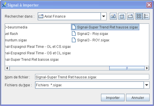In the signals library, imported signals are identified by the symbol

5. Strategy applied to a price chart

5.1. Generalities

A strategy can be applied directly to a price chart over a determined period. This operation is generally called backtesting.

Axial Finance offers the possibility of plotting the equity curve in the main chart of the prices in the selected chart window in the Market Tracking area, or plotting this equity curve in a secondary chart. Information regarding position opening and closing as well as the maximum drawdown can also be displayed in the chart.

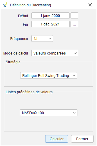
The strategy can be applied to the entire chart or between two specific start and end dates.

5.2. Customizing backtest result display in the chart

To customize the display of the backtest result in a chart, in the general Preferences menu, choose the option Strategy Charts to open the dialog window below. Select the Market Tracking tab:

Customization concerns both the equity curve traced in the main chart and that traced in a secondary chart.
To keep backtest results in memory, check the Keep backtest result box, otherwise these results will be lost upon closing the application.
To command the plotting of the equity curve in the main chart, check the Show Equity Curve box.

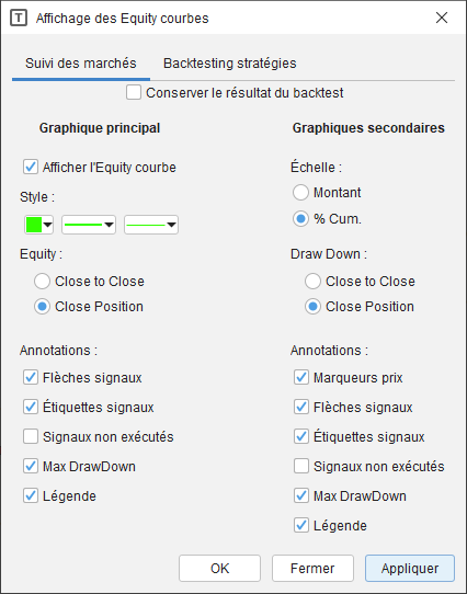Vertical scale for the Equity curve:
1. In the case of the main chart, the vertical scale of the equity curve is always in monetary units.
2. In the case of a secondary chart, one can choose between an amount-based scale (check Amount) or as a percentage of cumulative gains (check % Cum.)
The meaning of the percentage of cumulative gains is as follows: At each position closure, the gain (or loss) is calculated as a percentage of the opening price of that position. These gains (or losses) are then accumulated. This method of evaluating results avoids artificially inflating the result when, over the duration of the backtest, a large price variation occurs.
One can choose to plot or not, during position opening, the potential value of the equity curve at each bar. These are the two modes: equity in "Close to Close" or in "Close Position".
To request vertical arrows designating position opening and closing, check Signal Arrows.
To have the nature of the position ("long" or "short") and the number of shares displayed next to the previous arrows, check Signal Labels.
When a position is open, new opening signals remain without effect. Similarly when a position is closed with new closing signals. These unexecuted signals can be indicated on the chart as dotted arrows. Check the Unexecuted Signals box.
The maximum drawdown can be inscribed on the chart. Check the Max DrawDown box.
A legend recalling the executed strategy can also be inscribed. Check the Legend box.

5.3. Commanding backtesting

To perform a backtesting, open the strategy editing window by choosing in the general Trading System menu the option Edit Strategies.

Select the strategy from the library and click on the Apply button.

The window shown here opens to specify the period over which the strategy must be applied: the entire chart history (check Chart Dates) or from date to date (check Specific dates and define start and end dates).

Then click on Calculate to execute the strategy.

5.4. Equity curve in the main chart

Example of obtained plot:

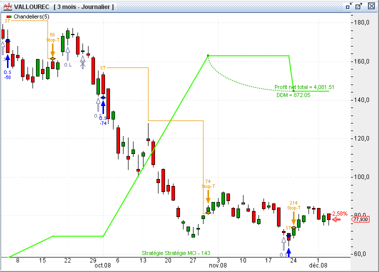
Symbology of the different information inscribed in the chart:

	Indicates the presence of a position opening signal with the indication O.L if "long" or O.S if "short" (note: this arrow is only visible if the position opening is delayed relative to the signal).
	Indicates that the position opening condition could not be executed and that the signal of opening is therefore cancelled because the validity period has expired.
	Indicates the effective opening of a position in "long" when the condition is met.
	Number of shares bought at the opening in "long".
	Indicates the effective closing of a position in "long" when the condition is met.
	Number of shares sold at the closing in "long".
	Indicates the effective opening of a position in "short" when the condition is met.
	Number of shares sold at the opening in "short".
	Indicates the effective closing of a position in "short" when the condition is met.
	Number of shares bought at the closing in "short".
	Closing a position on a stop.
	Type of stop: O on profit target, Lon maximum loss, T on profit loss, I on inactivity, E on end of day, M on maximum number of periods, B on break even.

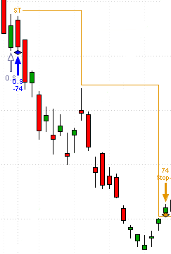Representation of the evolution of a trailing stop: The orange line indicates the level of the trailing stop at each bar. In this example, we can see that:

A position is opened in "short" at the bar following the detection of the signal.
A first level of the trailing stop is determined according to the formula.
The level of the trailing stop is then modified twice.
The position closure occurs as soon as the price breaches the trailing stop level.

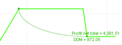Representation of the evolution of the invested capital (equity curve) and the maximum drawdown:

The green curve indicates the evolution of the invested capital with at its rightmost end the net total profit.
A dotted arc joins the extreme points of the drawdown, with the value of the maximum drawdown (DDM).

5.5. Equity curve and drawdown in a secondary chart

To display these curves in a secondary chart, one must add the indicators named Equity curve and Max Drawdown from the list of indicators.

Also specify the information to be displayed in these charts as indicated in the paragraph Customizing backtest result display in the chart above. In particular, two settings are important for analysis:

The vertical scale of these charts can be set in monetary units or as a percentage of cumulative profits. Check Amount or % Cum.
The drawdown curve can be displayed in Close to Close or in Peak to Valley. Check Close to Close or Close Position accordingly.
- In the first case, during position opening, the drawdown remains at its value from the moment of opening. Upon position closure, its value is then updated.
- In the second case, the potential drawdown is calculated with the lowest prices of each bar and displayed during position opening. A maximum drawdown in Peak to Valley mode allows one to know the real risk of maximum losses as long as the position is not closed.

6. Analysis of strategy results

6.1. Generalities

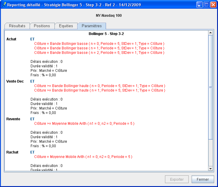
Axial Finance presents the numerical results of strategies in three different forms:

A General report for all trials related to a single strategy and for a given stock.
A detailed report for each trial.
A global table of all trials performed or kept in memory with all the strategies and for all stocks.

6.2. General report of strategy trials

Once the backtesting operation is performed, click on the Report button in the strategy editing window. A new window opens providing a list of all trials performed with this strategy:

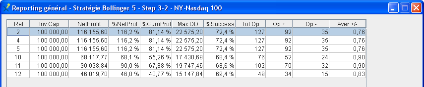
This general reporting table summarizes the main results of each trial for a single stock:

Ref	The reference number of the trial
Inv. Cap.	The reminder of the initial capital invested or required to apply the strategy
Net Profit	The realized net profit
% Net Pro.	The percentage of net profit realized relative to the initial capital invested
% Cum. Pro.	The percentage of cumulative gains (or losses)
max DD	The maximum drawdown (in monetary units)
% Success	The percentage of success (ratio of winning positions to the total number of positions)
No. Trades	The total number of positions
Win Trades	The number of winning positions
Loss Trades	The number of losing positions
Avg G/L	The ratio of net gains to net losses

6.3. Detailed report of a strategy trial

To access the detailed report of the trial, select it from the list in the general reporting window and click on the Detail button, or double-click directly on the trial in the list.

Another window opens allowing you to consult the following four reports:

6.3.1. Results

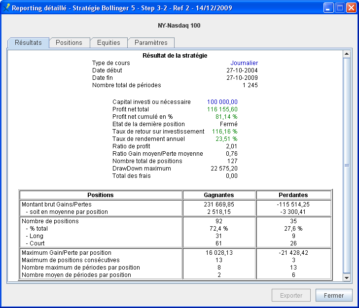
This first table presents the various calculated ratios. It also specifies the start and end dates of the trial, the nature of the prices and their periodicity, as well as the status of the last position if it is still open.

6.3.2. Positions

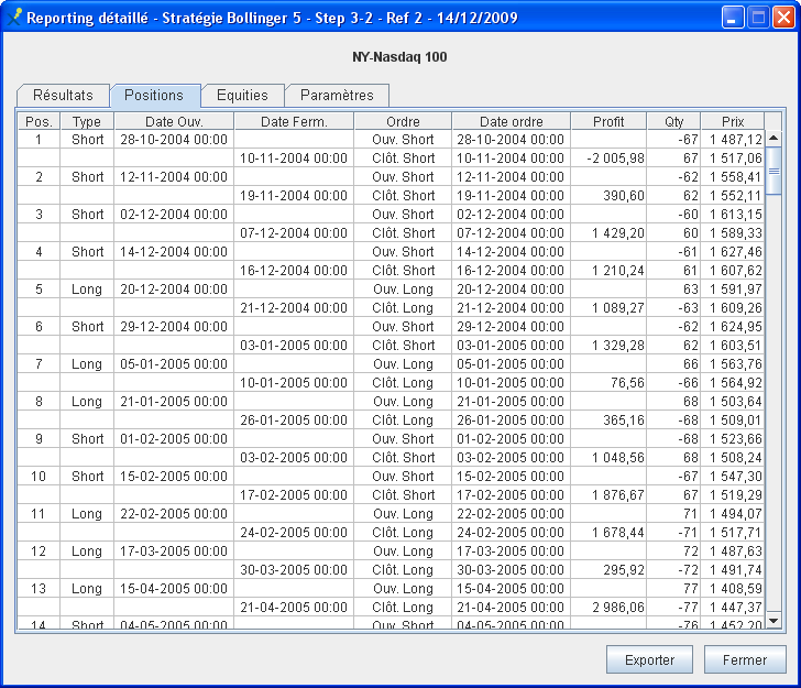
This second table provides the list of all positions that were opened, with for each position:

Its nature, "long" or "short"
The type of order placed to open and close the position
The opening and closing dates
The realized profit or loss
The number of shares
The order price at opening and at closing

6.3.3. Equities

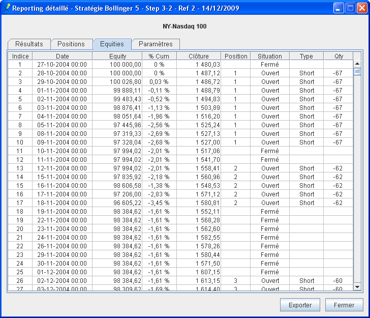
This third table provides the list of the equity at each bar specifying:

The date
The equity value
The cumulative percentage of profits (or losses)
The closing price
The reference number of the open position
The status of the position
The type of the open position
The number of shares

6.3.4. Parameters

This fourth table recalls the strategy applied along with the parameters and conditions of the trial.

6.4. General tables for all strategy trials

All trials performed during the session or kept in memory for all strategies and for all stocks are viewable in two tables present in Strategy Screen: The table titled Global Report and the one titled Optimization Report.

To access these tables, select Strategy Screen at the top of the screen then the Global Report tab or the Optimization Report tab.

6.4.1. Global Report

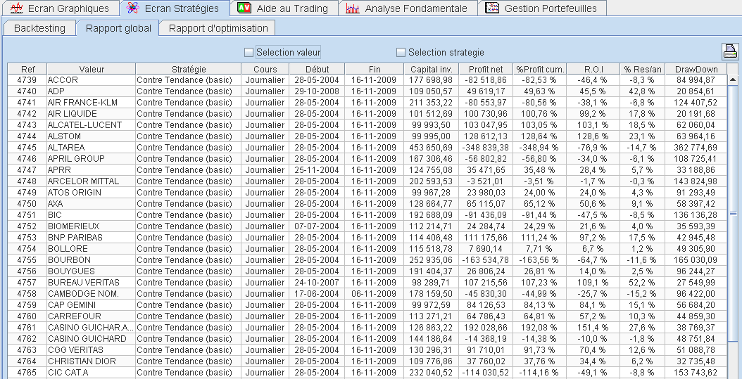
This table displays the main results of each trial.

It allows for the following operations:

Access the detailed report of the trial by double-clicking on the corresponding line.
Sort the table rows according to result ratios: Double-click on the column header.
Reduce the table to trials for a single stock: Select a row with that stock and then check the Select Stock box at the top of the table.
Reduce the table to trials for a single strategy: Select a row with that strategy and then check the Select Strategy box at the top of the table.
Clear results: select the result row(s) to clear and then press the Delete key on the keyboard, or open the context menu by right-clicking and choose the Clear option.

6.4.2. Optimization Report

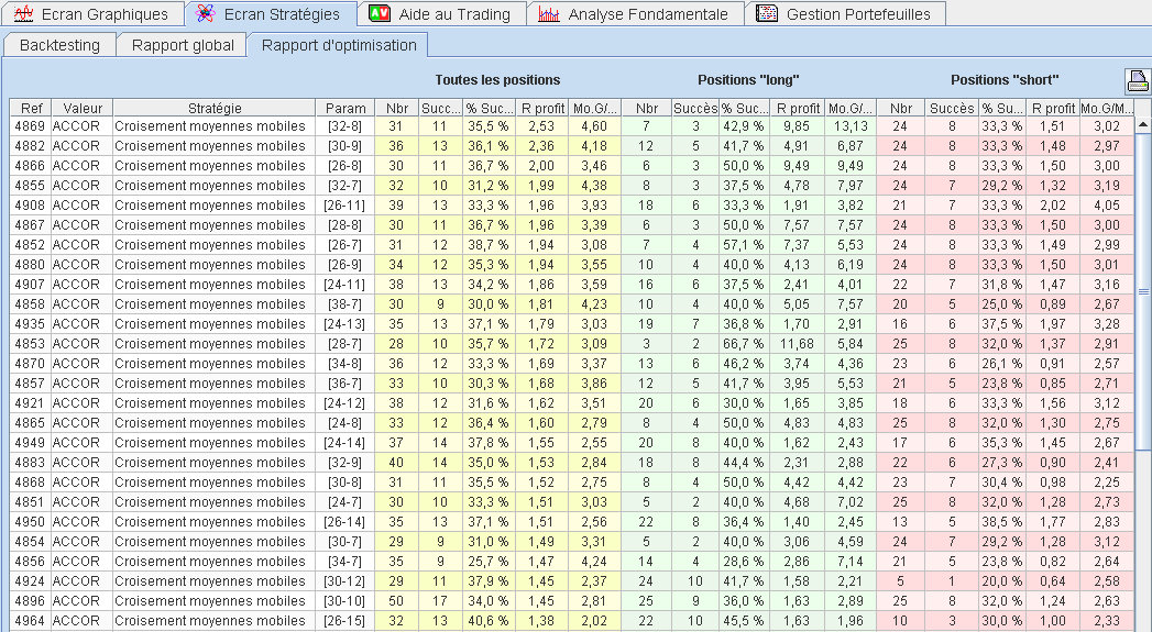
This table is specifically dedicated to comparing the results of a strategy applied to a stock, a strategy whose parameters vary according to a variability profile defined by the user (see the paragraph below Defining parameter variability).

This table indicates for all trials:

in the param column, the set of parameters applied
and for all open positions, in particular in the cases of Long and Short:
1. The total number of open positions in the Nbr column
2. The number of winning positions in the Success column
3. The % of winning positions in the % Success column
4. The profit ratio in the R profit column
5. The ratio of average wins over average losses in the M.W/L P. column

To obtain the set of parameters providing the best result, click on the R profit column header to sort trials by descending profit result.

7. Comparison of strategies

7.1. Generalities

In the Strategy Screen module, Axial Finance simultaneously applies one or more strategies to one or a set of stocks in order to obtain on a single chart the plots of the equity curves and the maximum drawdown.

Three modes are available:

The mode called Stocks compared: a single strategy is applied to a list of stocks,
The mode called Strategies compared: several strategies are applied to the same stock,
The mode called Variable parameters: a single strategy is applied to a stock, while step-by-step varying the parameters of the indicators contained in the rules of this strategy.

Detailed results are available in the global trials table.

7.2. Customizing strategy result display in the chart

To customize the display of the result in Strategy Screen, in the general Preferences menu, choose the option Strategy Charts to open the dialog window below. Select the Strategy Screen tab:

To retain the results of the strategies in memory, check the Keep backtest result box; otherwise these results will be lost when the application is closed.
In order to compare results across securities, the vertical scale is set by default as a percentage of cumulative gains. The meaning of cumulative gains percentage is as follows: Each time a position is closed, the gain (or loss) is calculated as a percentage of the opening price of that position. These gains (or losses) are then accumulated.

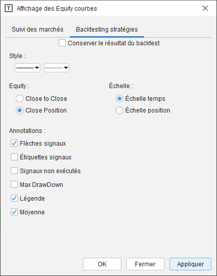You can choose whether or not to plot the potential value of the equity curve at each bar while positions are open. These are the two modes: Equity in "Close to Close" or in "Close Position".
The horizontal scale can be proportional to time (check Time Scale) or proportional to the number of positions (check Position Scale).
To request the drawing of vertical arrows indicating the opening and closing of positions, check Signal Arrows.
To display alongside the above arrows the type of position ("long" or "short") and the number of shares, check Signal Labels.
When a position is open, new opening signals have no effect. Likewise, when a position is closed, new closing signals have no effect. These unexecuted signals can be plotted on the chart as dashed arrows. Check the Unexecuted Signals box.
The maximum drawdown can be displayed on the chart. Check the Max DrawDown box.
A legend recalling the strategy that was run can also be displayed. Check the Legend box.
To display the average of the equity curves shown in the chart, check the Average box.

7.3. Choice of comparison conditions and launching the trial

Click on the Choose button at the top left of Strategy Screen to open the dialog window below:

Fix the start and end dates.
Specify the nature of the prices to use: "end of day" in Daily, Weekly or Monthly or Intraday with the desired periodicity.
Choose one of the three calculation modes, and then according to the mode:
- With the Stocks compared mode, select the strategy to apply from the drop-down list Strategy as well as one of the stock lists in the third drop-down list.
- With the Strategies compared mode, select the stock to use from the Stock drop-down list as well as the strategies by checking those requested.
- With the Variable parameters mode, select the stock to use from the Stock drop-down list as well as the strategy to apply. Then, to define parameter variability, see the following section.

Then, to launch the calculation, click on the Calculate button in this window or on the one located at the top right of Strategy Screen.

7.4. Defining the variability of rule parameters

To define the variable parameters in a rule of a strategy :

Open the strategy editing window by choosing in the general Trading System menu the option Edit Strategies.
Select the strategy from the library and then the rule in which the signals are to be parameterized.
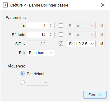
Double-click on the signal in the rule to open the parameter entry window.

Example of a signal parameter entry window:

To obtain a variable parameter, check the box next to this parameter and choose the variability profile from the associated drop-down list.
To create a new variability profile or to modify an existing one, click on the ... button to open the window below.

Variability profiles definition window:

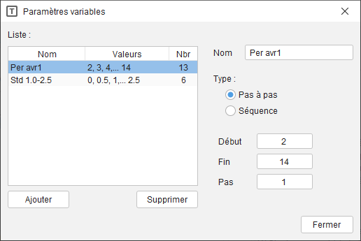Axial Finance provides two types of profiles:

Either step-by-step between two extreme numbers
Or according to a sequence of discrete numbers

Click on the New button to add a profile, enter the profile name, choose the type and the various parameters defining the variation.

During trial execution, all combinations of numerical values of the variable parameters are successively taken into account. The number of charts obtained is equal to this number of combinations. The chart legend indicates the set of parameters corresponding to each curve.

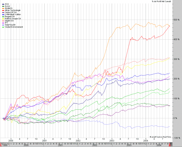
7.5. Presentation of comparison in a chart

In the example above, a strategy was applied to a list of 12 stocks. The vertical legend on the left provides the list of these stocks.

By selecting a stock in the legend, the corresponding equity curve is highlighted by small rectangles.

By selecting a curve in the chart, the name of the stock in the legend is enclosed in a black frame.

By double-clicking on an equity curve or the stock name in the legend, the detailed report presentation window opens.

An equity curve can be removed from the chart: Select this curve and then open the context menu by right-clicking and click on the Delete option. In this case, the average curve (if displayed) is automatically recalculated.

Prev		Next
Chapter 6. Fundamental Analysis	Home	Chapter 8. Order Placement